If you need to dynamically calculate values that are dependent on other values entered in your worksheets, then you need formulas. Formulas will calculate values for you so that you don’t have to spend time struggling with Maths and risk making mistakes. In Excel 2010, you can use formulas to calculate things like:
- Total household expenditure
- Loan repayments
Cell Reference
To create a formula that uses data in certain cells, you’ll need to refer to those cells. In Excel, cell references are given by supplying the column letter and row number. For example, cell C3 exists at the intersection of column C and row 3.
A Simple Formula – AutoSum
To start things off, let’s look at an example using a formula that provides a total amount.
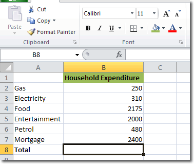
In the total row, we want to display the sum of all household expenditure. Make sure that the cell you want to contain the total is active and then click Home > Editing > AutoSum. Because the active cell is positioned directly below a column of numbers, Excel 2010 guesses that you want to sum them and places a selection around them (see A below).
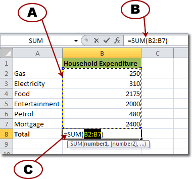
B is called the Formula Bar and it displays the content of the active cell, which in this case is a formula. C is the active cell and contains the formula. Let’s look at the structure of a formula.
You can see that the formula starts with a “=”. All formulas must start with “=”. The next part is SUM, which you can guess represents the SUM function. The contents of the brackets are called arguments and they define the range of cells that we are summing – in this case cells B2 to B7. This range is defined as B2:B7. Autosum is a quick and easy formula to use that automatically identifies its input variables. Let’s now look at a formula we can set up manually.
Defining Your Own Formula In Excel
Suppose we have the following example that details price, VAT and total price.
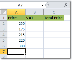
As you can see, we start with a price before VAT and we need to calculate first the VAT and then the total price. Let’s calculat the VAT first, based on a VAT rate of 17.5%. The formula therefore is VAT = 17.5% x Price. Make cell B2 active and in it type
=17.5%*A2
Excel knows how to handle percentages so you don’t need to convert 17.5% to 0.175 for the calculation. When you press enter, Excel calculates the VAT to be 43.75. We have dealt with the first VAT amount, but what about the rest? There is a quick and easy way to apply the formula you just created to other cells. With cell B2 active, position the cursor over the bottom right corner so that the cursor becomes a ‘+’. When it does, drag downwards to select all cells that should use the formula (down to cell B6).
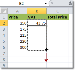
When you release the mouse, Excel applies the VAT formula to the selected cells and calculates their values. That’s the VAT for all rows take care of. On to the total price.
Total price = price + VAT
We can define that as a formula by typing into C2 the following
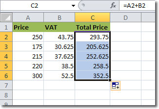
=A2+B2
When you press Enter Excel calculates the sum of A2 and B2 to give 293.75. And we’ve already seen how we can to apply that formula to the remaining cells. The finished spreadsheet should look like this.
