New to Microsoft Excel 2010 are Sparklines. Sparklines are simple and compact graphs that show trends. Their small size means that sparklines can fit inside a single cell to give you “at a glance” information about your data. If you need to present trends very clearly in a small space, then sparklines are an ideal solution.
Sparklines were developed by Edward Tufte to give a simple, condensed way to present trends and variation, associated with a measurement such as average temperature or stock market activity.
Open up the worksheet and then click in cell G3 to make it active. We’re going to insert a sparkline in this cell that represents the monthly fuel bills to its left. It helps to position a sparkline near its data for greatest impact. With G3 active, click Insert >Sparklines > Line.

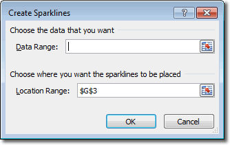
Excel has already identified cell G3 as the Location Range because that was the active cell. We now need to tell Excel what data to use for the sparkline, and we can do that by selecting cells A3 to F3. When these cells are selected, Excel puts A3:F3 into the Data Range box. Click OK and a line sparkline is created.

Whereas charts in Excel are objects, sparklines are actually placed in a cell’s background. This means that you can enter text in a cell and use the sparkline as its background. For example, we could type some text into cell G3 and the sparkline would act as its background. Some people may not like the way that text inserted in this way obscures the tiny sparkline.
There aren’t many formatting changes we can make to this sparkline, but let’s make some that may prove useful. Let’s add some markers. With cell G3 active, you should see the Sparkline Tools tab in the ribbon. Click Design > Style > Marker Colour > High Point, and select a colour that contrasts with the line colour. Do the same for the Low Point too.

To delete a sparkline from a cell, pressing the delete key will do you no good! This is because the sparkline is in the cell’s background. Instead, you need to click the Clear button on the Design tab.
Let’s leave the line sparkline where it is and create a column sparkline below it so that we can compare them. Make cell G4 active and click Insert >Sparklines >Column. Select the data cells again and click OK. Now, we have the following sparklines:

If you decide to change the sparkline’s type, you can simply click on the one you want in the Type group on the Design tab. The sparkline will immediately change to that type.

