Excel PivotTables (pivot tables) enable us to extract meaningful information from large volumes of apparently meaningless data. Using PivotTables, we can “pivot” our data to view it from different angles to give us more useful insights. As you will see, you will soon be able to quickly discover the trends and patterns that are buried deep within your data.
Once you have the worksheet open, click into any cell within the data. To create a PivotTable, click Insert > PivotTable. The Create PivotTable window opens for you to confirm the cell range selection and to select whether to create the PivotTable in the current worksheet or a new one. Ensure that New Worksheet is selected and click OK.
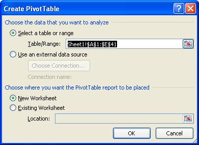
A new worksheet will open and the PivotTable is inserted on the left, whilst the PivotTable Field List is displayed on the right. The PivotTable doesn’t display anything just yet because we haven’t yet selected any fields from the field list.
Selecting Fields From The Field List
Select the following fields from the top of the Field List by checking their boxes and watch where they appear:
- Region
- Date
- Software Sales
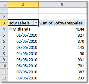
You should end up with a PivotTable that looks like this:
and a Field List that looks like this:
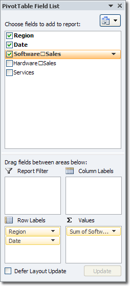
When you select fields from the field list, they will appear in the Values section if they are numeric and they will appear in the Row Labels section if they are non numeric or are dates. That is the reason why Region and Date appear as Row Labels. Also, as Region was selected first, it becomes the outer row field, while Date becomes the inner row field. Software Sales, being numeric, appears in the Values area of the field list, and in the actual data part of the PivotTable.
However, you can move the fields around by dragging and dropping them into the area where you need them. In our example, the data might be more readable if we display the values in a new column for each region. To this end, move the Region data field to the Column Labels area by dragging and dropping it there in the PivotTable Field List. You could also click on the field and select Move To Column Labels.
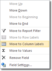
Notice how the PivotTable updates its structure immediately. The new layout looks much better (click on the image to expand).
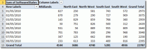
Notice also that Excel automatically calculates totals: there are row totals for each date across all regions, and there are also totals for each region across all dates.

