The explanation for how VLOOKUP works in Excel is far more complicated than actually using it. The best thing to do is to get a rough idea of the arguments that VLOOKUP requires, and what it returns to you, and then quickly go on to look at a few VLOOKUP examples.
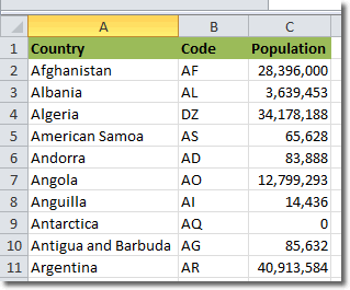
Imagine you have the following spreadsheet:

In this example, you need Excel to give you the country code if you give Excel the country. It’s helpful to break down what you as a human would do to complete this task. Let’s get the country code for Angola now.
- State what we are searching for, and that is the text “Angola”
- Then we identify what table contains the data we need, and that’s A2:B11.
- Then we determine what column holds the information we need Excel to return to us, and that’s column 2 (country code).
These three pieces of information are precisely what Excel needs to perform the VLOOKUP, and they are provided in the following format:
VLOOKUP(search_value, table_array, column_to_return)
So, to get the country code for Angola, we would use the following VLOOKUP:
=VLOOKUP(“Angola”, A2:B11, 2)
Don’t forget the “=” at the beginning of the formula.
The above example shows the most basic way of using VLOOKUP, and it returns an exact match on the country code. If “Angola” couldn’t be found in the table, Excel would return #N/A. We can, however, provide an additional parameter to Excel’s VLOOKUP: not_exact_match. The format then looks like:
VLOOKUP(search_value, table_array, column_to_return, not_exact_match)
not_exact_match takes the value TRUE or FALSE. If set to FALSE, Excel tries to find an exact match. If set to TRUE, Excel finds the largest value in column 1 that is less than or equal to the search value. Imagine we were trying to get the country code for the fictional country “Amporo”, which doesn’t exist in the table. Here, it only makes sense to look for an exact match, so we would use:
=VLOOKUP(“Amporo”, A2:B11, 2, FALSE)
Excel would return #N/A because “Amporo” doesn’t exist in the table. If, instead we used:
=VLOOKUP(“Amporo”, A2:B11, 2, TRUE)
then Excel would return AS. American Samoa is the largest value less than or equal to Amporo, so AS gets returned.
Now that we’ve seen VLOOKUP in action, let’s visit the official definition:
VLOOKUP searches for a value in the first column of a table array and returns a value in the same row from another column in the table array.
The V in VLOOKUP stands for vertical. Use VLOOKUP instead of HLOOKUP when your comparison values are located in a column to the left of the data that you want to find.
Have a look at this illustrative VLOOKUP example.

