If you have a large table of data in Microsoft Excel and you scroll down, it can be hard to remember what each column represents. This problem becomes exacerbated when you have a large number of columns and the data in each is of a similar size. How do you remember what each number means?
You don’t need to.
When you freeze panes, you keep specific rows or columns visible when you scroll in the worksheet. This means that if your table has column headings – or even row labels – you can freeze them in place so that you can always see them when you scroll.
Depending on what you want to freeze, do the following:
- To freeze rows, select the row below the row or rows that you want to keep visible when you scroll.
- To freeze columns, select the column to the right of the column or columns that you want to keep visible when you scroll.
- To freeze both rows and columns, click the cell below and to the right of the rows and columns that you want to keep visible when you scroll.
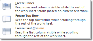
Then click View > Window > Freeze Panes.

Now do one of the following:
- To freeze one row only, click Freeze Top Row.
- To freeze one column only, click Freeze First Column.
- To freeze more than one row or column, or to freeze both rows and columns at the same time, click Freeze Panes.
When you want to unfreeze panes, click View > Window > Unfreeze Panes

